Project:Computational Statistics to Understand Bias in Handwritten Digit Predictions
The final project paper is now available online at my GitHub Repo
Introduction
This is a project repo of Umich 2022-2023 Fall course STATS406, using computational statistical methods to analyze potential bias in hand-written digit prediction process. Specifically, the research utilizes computational statistical methods to investigate the potential influence of object size and shape in image classification, specifically in the context of the MNIST dataset. The motive behind this work is to address the challenge of biases in machine learning models, particularly the potential model bias from different object shapes and sizes.
Data Collection
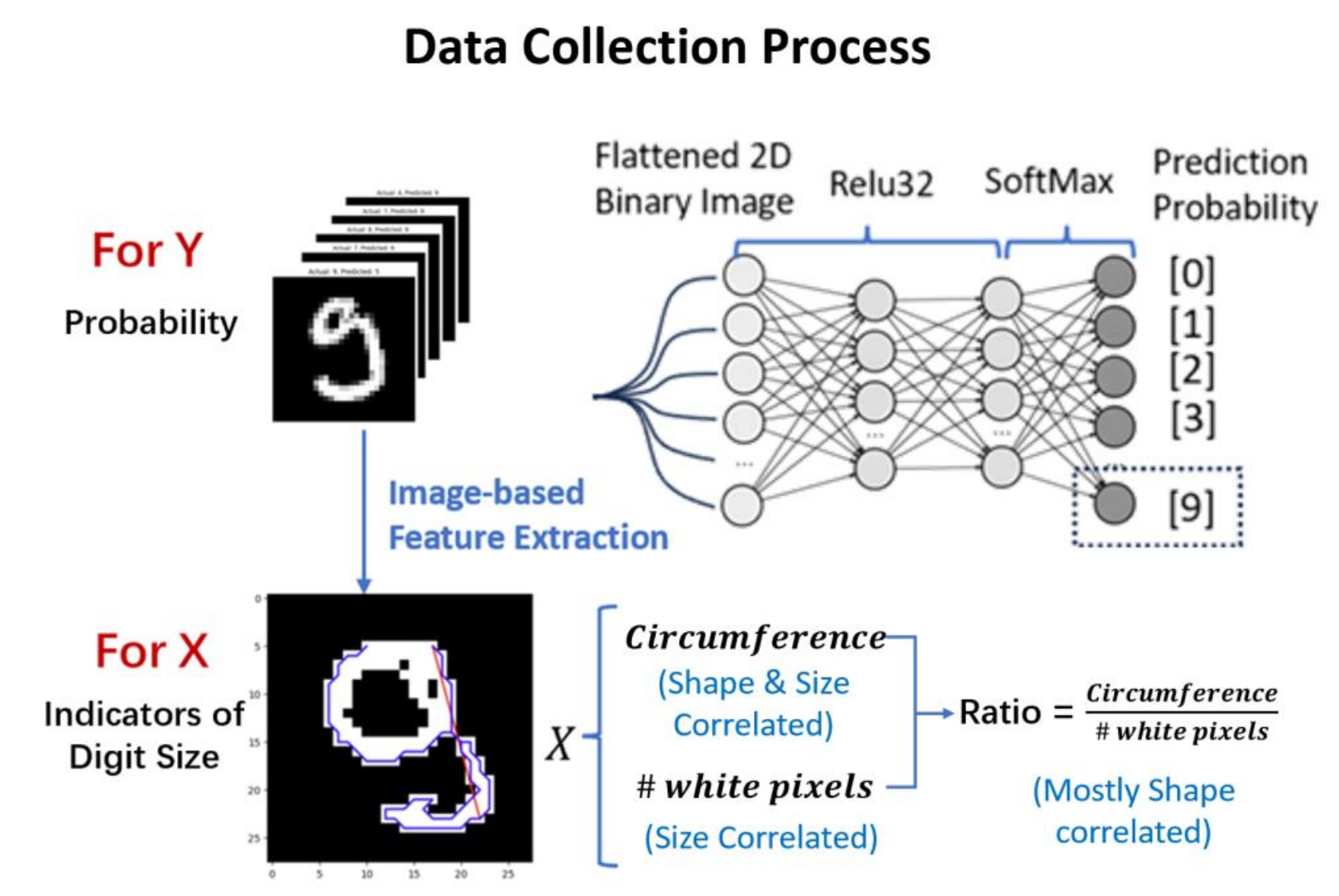
The data collection process involves the use of the MNIST Database, a widely used benchmark dataset in the field of machine learning and computer vision, which consists of 60,000 training examples and 10,000 test examples of handwritten digit images. The images in the MNIST dataset have been preprocessed, including normalization and centering, resulting in a fixed-size image of 28x28 pixels. To indicate the shape and size of different handwritten images, the following features are extracted from the image:
Size
\[Size =\frac{\text{# White Pixels}}{\text{# Total Pixels}}\]This feature mainly calculated the portion of the area that the digit takes with respect to the total number of pixels of the image, which is constant 768 for all cases.
Circumference
\[\begin{gathered} \text { Boundary Points } \epsilon=\left\{\sigma \mid \operatorname{Point}[\sigma]=1 \wedge \bigcup_{\text {dir }} \operatorname{Point}[\sigma+\operatorname{dir}]=0\right\} \\ \text { Circum }=\sum_{(i, j) \in \epsilon} \| \text { Point }[i]-\operatorname{Point}[j] \|_2 \end{gathered}\]We consider circumference as one of the factors to be taken into account when establishing the model, as it can distinguish the writing of certain digits. In cases where the sizes are similar, digits with more complex strokes such as 4, 5, 8, 9, etc., are considered to have a larger circumference.
Ratio
\[\text { Ratio }=\frac{\text { Circum }}{\# \text { white pixels }}\]When the original digit is zoomed, the circumference and size would change proportionally at the same time, and the ratio would remain unchanged. Therefore, in the context of following analysis, we could assume as a mostly shape-correlated feature, as a size-dominant one, and the is mutually influenced by shape and size of the digits.
Methodology
Bootstrapped Skewness Diagnostics
To assess the skewness of the features extracted from the MNIST dataset, we employ bootstrapped skewness diagnostics. Skewness is a statistical measure that describes the asymmetry of a probability distribution about its mean. A skewness value of 0 indicates a perfectly symmetrical distribution, while positive or negative values suggest a skew to the right or left, respectively. In the context of skewness diagnostics, bootstrapping provides a robust method for estimating the skewness of the features and assessing its variability.

Stratified Sampling & Permutation Test
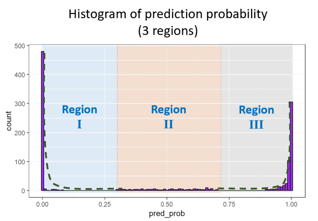
The normality assumption of extracted image features is based on the common fact that the way people are taught to write digit should be largely similar for other people to recognize. However, when it comes to the prediction probability, the neural network is well-trained to binarize the classification probability. In this respect, we should expect a fairly large frequency appearing at the low end (probability close to 0) and high end (probability close to 1) of the prediction probability. Therefore, the original normality assumption does not hold anymore. A histogram visualization of the prediction probability suggests that the first and the last bin have the largest sample frequency, and the number of samples decays in an exponential shape when the prediction probability gradually approaches 0.5. Since the probability is defined on the [0,1] region, we can use truncated exponential distribution for each region to express the probability distribution at both ends.
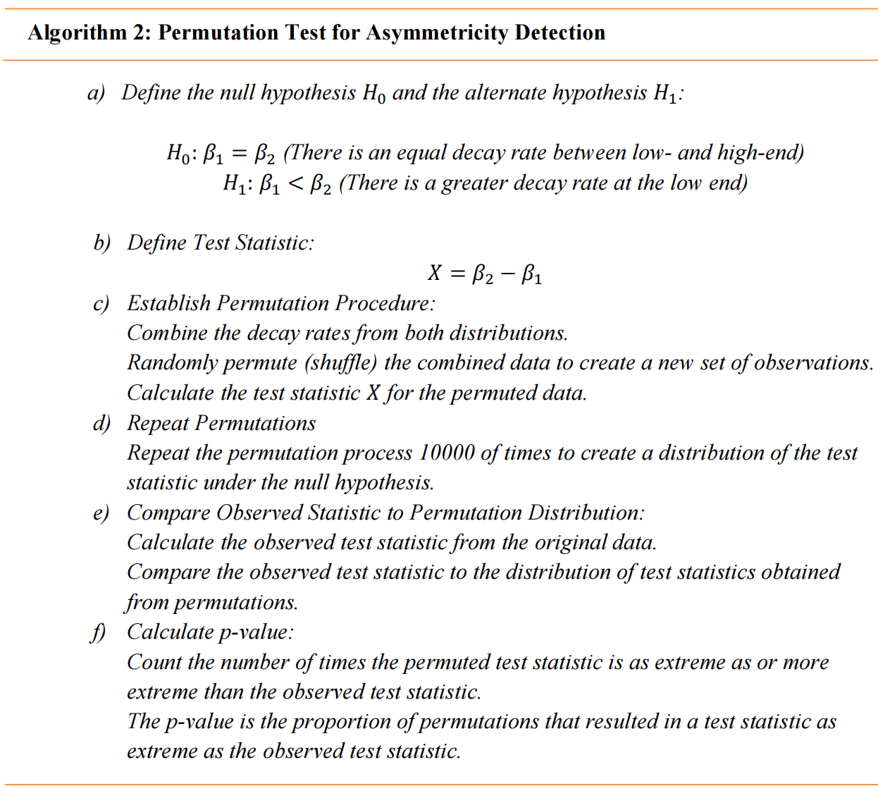
To detect whether the symmetric assumption is valid or not, we employ the permutation test as follows:
Result & Analysis
Global Normality
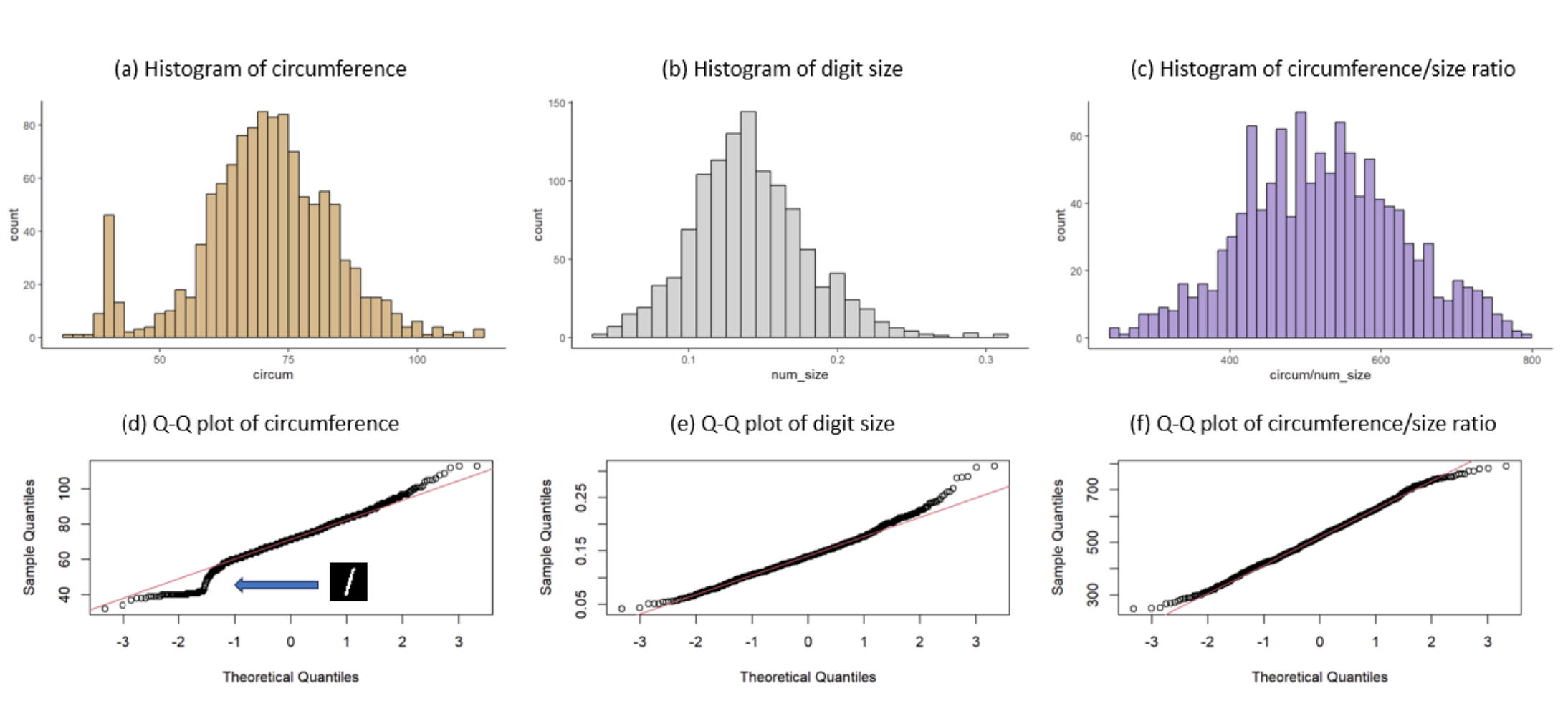
The extracted features of all digits together form a normal distribution
Bootstrapped Feature Distribution
After successfully sampling the data on each stratified region, we perform bootstrapping to compute the conditional mean & variance for three regions together with the confidence intervals. The kernel density plots of the mean statistics of the bootstrapped sample (bootstrapped sample distribution) are presented in the following figure.
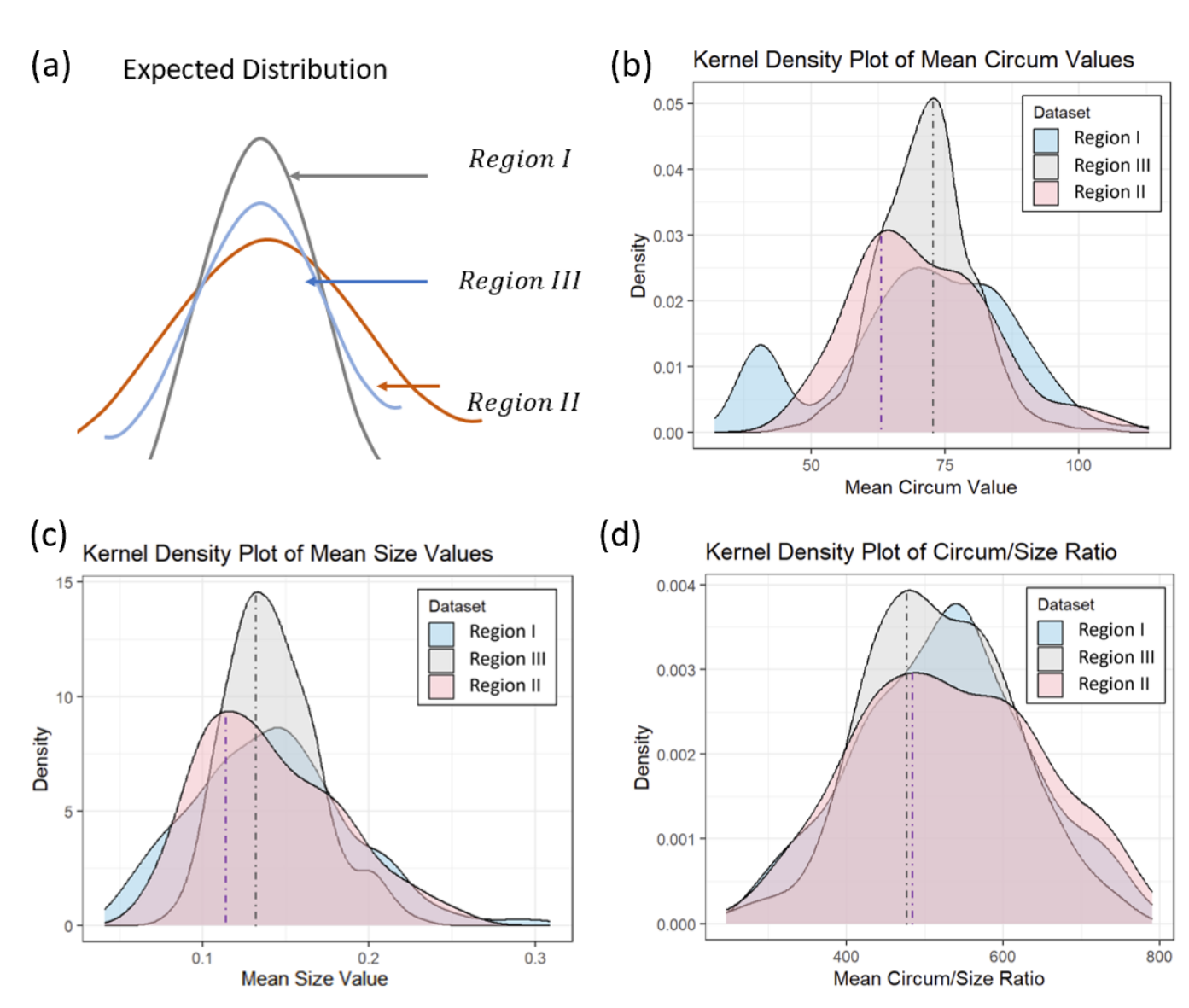
In expectation, in order to suggest that there is no evident bias in the model prediction result, the feature statistics should satisfy:
\[\begin{gathered} \operatorname{Mean}(\cdot \mid \operatorname{Region} I I I) \approx \operatorname{Mean}(\cdot \mid \operatorname{Region} I) \approx \operatorname{Mean}(\cdot \mid \operatorname{Region} I I) \\ \\ \operatorname{Var}(\cdot \mid \operatorname{Region} I I I)<\operatorname{Var}(\cdot \mid \operatorname{Region} I)<\operatorname{Var}(\cdot \mid \operatorname{Region} I I) \end{gathered}\]The expected condition only occurs for the feature Ratio, which is a shape-correlated feature. When it comes to size correlated features Size and Circumference, although the mean value still approximates for three regions, the variance of Region I exceeds that of Region II. Moreover, the kernel density plot reveals that the peaks of the Region II has been deviated from the peak of Region I. To further understand the underlying reason, we turn to a detailed observation of each digit and examine whether our previous normality assumption still holds true when it comes to separate digit.
Local Normality
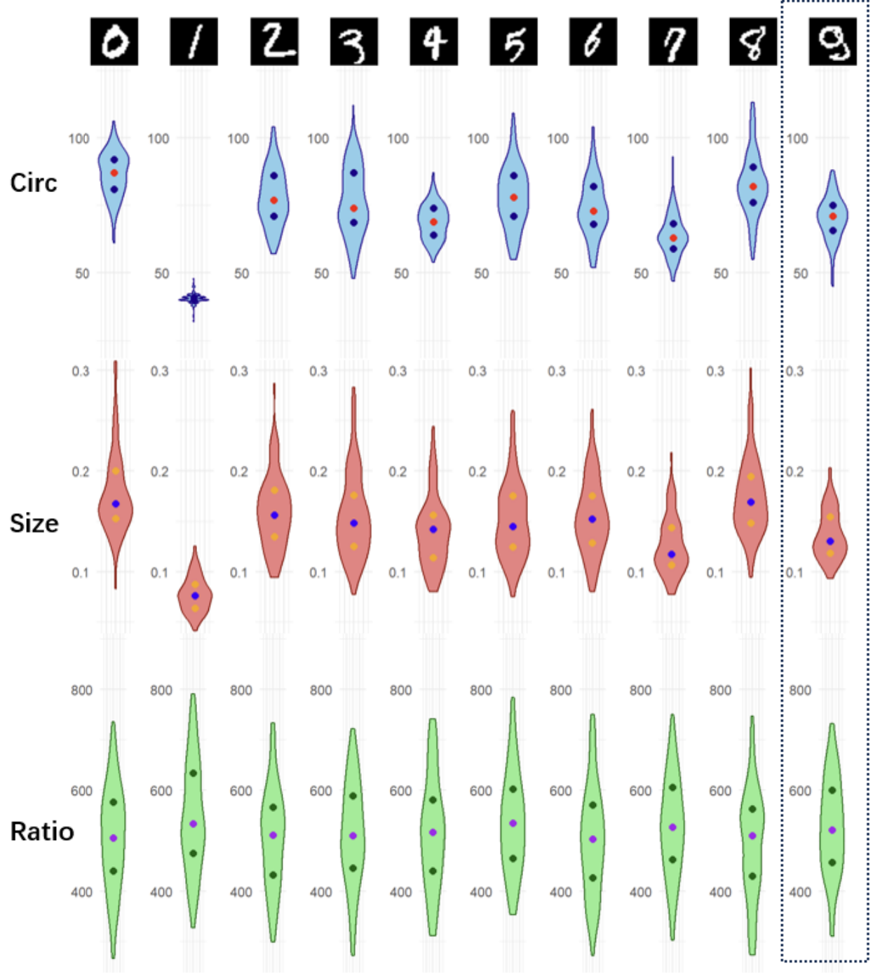
To determine whether our previous normality assumption still holds true when it comes to separate digit, we visualize the distribution using violin plot as shown in the following figure.
Bootstrapped Skewness Test Result
| Statistics | 0.95 Confidence Interval | |
|---|---|---|
| Circum | -0.37 | [-0.97, -0.12] |
| Size | 0.57 | [0.26, 0.99] |
| Ratio | -0.004 | [-0.34, 0.33] |
Unlike shape-related features, which demonstrate a normal distribution for each individual digit, the size-related digits exhibit inconsistent distributions across different digits. This inconsistency perpetuates a non-normal distribution for each digit, juxtaposed with an overall appearance of normality.
Conclusion
The comparison between global normality and local normality highlights a key finding from the research, indicating that while shape-related features demonstrate a normal distribution for each individual digit, the size-related features exhibit inconsistent distributions across different digits, leading to a non-normal distribution for each digit, despite an overall appearance of normality.
This inconsistency in the distribution of size-related features across different digits suggests that the impact of object size on the model’s predictions varies significantly depending on the specific digit being analyzed. In other words, the influence of size-related features on the model’s decisions is not uniform across all digits in the dataset. Overall, this finding contributes to a deeper understanding of the potential biases introduced by size-related features in image classification models, and it underscores the need for continued research into more nuanced and effective methods for bias detection and mitigation in machine learning systems.
Notice: It should be noted that the code implementation of the calculate_power in the simulation section is flawed. The code is calculating the p-value of the statistics instead of the power. P-value is a statistics for the given data, which is deterministic, power is an indicator to evaluate the type-B error of the statistical method, which involved iterations. The overall analysis logic of the simulation section in this paper does not suffer from this code flaw.